Querying time series data
This is a blog post series focused on IoT
- Part I: Introduction
- Part II: Ingesting data
- Part III: Querying data (this post)
It’s now time to start playing with the data. In this post, I’ll run some of the most common query patterns we find in IoT projects on both Azure Data Explorer and TimescaleDb.
To recap: we have loaded a dataset of about 113 million rows of data to each database. For more details, read the previous blog posts (see links at the beginning of this post).
Let’s get ready to rumble
Count
Let’s first do a count across the entire dataset.
Table-wide counts are infrequent, and typically done for the internal purpose of understanding the magnitude of your dataset. However, this is a quick way to see if your data is properly indexed or if your database is keeping statistics in the background to speed up aggregation operations.
ADX
1
2
Trucks
| count
| Result | Execution time |
|---|---|
| 114,048,366 | 97 ms (that’s milliseconds) |
Timescale
1
SELECT count(*) FROM trucks;
| Result | Execution time |
|---|---|
| 113,000,115 | 1 minute 01secs |
The exact magic behind the ADX numbers are unknown to me (I’ll let the PG comment on that and enlighten us with the details), but I suspect ADX keeps some statistics or heuristics at hand to return a table-wide count in under 100 milliseconds for 114 million rows of data.
On the other hand, Timescale has difficulties with this query. Running a EXPLAIN ANALYZE on that query shows that, whereas the count at the chunk level (remember, this is where paralellisation happens) completes very fast, it’s the aggregation of the results that seems to take forever. Some people from the Timescale community have complained that Timescale on Azure Postgres suffers from slow disk performance (thanks Mario from PackIOT for the pointer), but even after increasing the IOPS on the database, the performance of the query can’t be brought down to less than 1 minute (the initial execution of this query prior to increasing the IOPS was about 3 minutes). See HERE for the issues with disks.
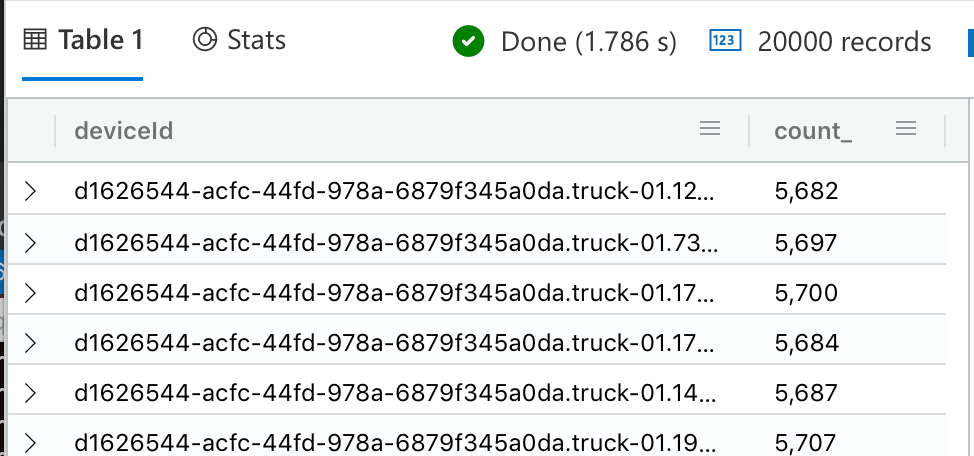
Grouping by DeviceId
Here, we’ll count how many unique DeviceId’s we have in the table, and count the number of messages per device.
Counting by deviceId is important. First, it lets you quickly identify the most active devices in the field. It also lets you detect anomalies (for example, a device that has always been quiet but is now sending messages out of control). It might also be your billing unit (you charge your users on a per-message basis).
ADX
1
2
Trucks
| summarize count() by deviceId
| Result |
|---|
|
| Execution time: 2.355secs |
Timescale
1
SELECT connectiondeviceid, count(*) FROM trucks GROUP BY connectiondeviceid;
| Result |
|---|
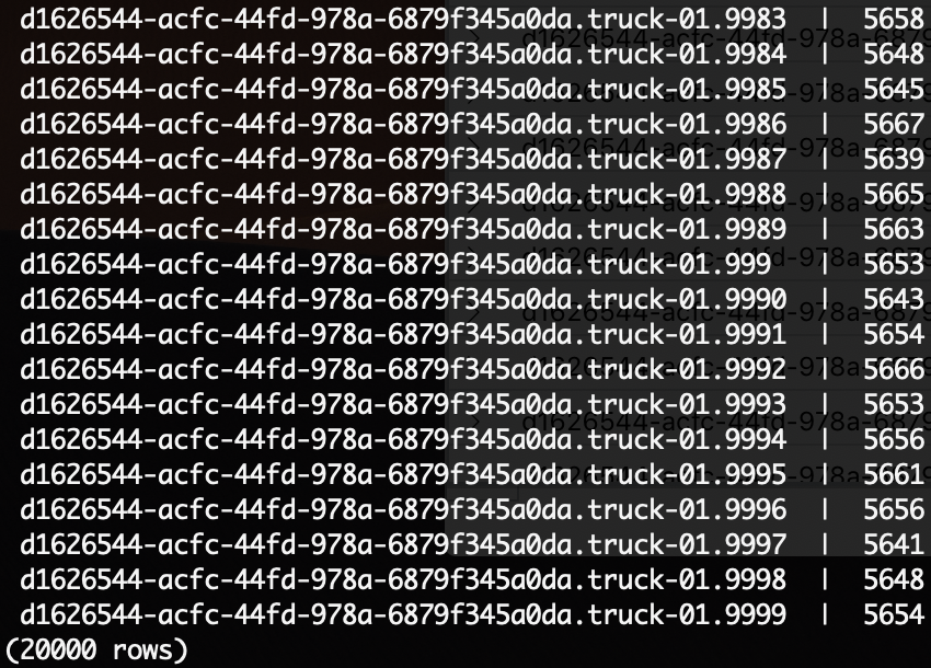 |
| Execution time: 1min 20secs |
Message count for 1 DeviceId
We will now pick one specific deviceId, and count the number of messages in the entire dataset. This is a very common metric to show your users, as it provides them a utilisation metric.
ADX
1
2
3
Trucks
| where deviceId == 'd1626544-acfc-44fd-978a-6879f345a0da.truck-01.11578'
| summarize count()
| Result |
|---|
| 5,698 |
| Execution time: 135 ms |
Timescale
1
2
SELECT COUNT(*) FROM trucks
WHERE connectiondeviceid = 'd1626544-acfc-44fd-978a-6879f345a0da.truck-01.11578';
| Result |
|---|
| 5,645 |
| 1.626secs |
We finally see Timescale coming back with a result within a reasonable timeframe. This is probably due to the low cardinality of the result set, since we are aiming for 1 single deviceId (instead of 20,000 in the past query). However, this query is complex in that it requires the database to activate all its partitions. This query benefits from indexing, as can be seen by the EXPLAIN ANALYZE command:
1
2
3
4
5
6
7
8
9
10
11
12
13
14
sampledb=> EXPLAIN ANALYZE SELECT COUNT(*) FROM trucks WHERE connectiondeviceid = 'd1626544-acfc-44fd-978a-6879f345a0da.truck-01.11578';
                                                                                               QUERY PLAN
---------------------------------------------------------------------------------------------------------------------------------------------------------------------------------------------------------
 Aggregate (cost=6333.61..6333.62 rows=1 width=8) (actual time=7.236..7.236 rows=1 loops=1)
   -> Append (cost=0.00..6319.68 rows=5570 width=0) (actual time=0.052..6.938 rows=5645 loops=1)
         -> Seq Scan on trucks (cost=0.00..0.00 rows=1 width=0) (actual time=0.004..0.004 rows=0 loops=1)
               Filter: ((connectiondeviceid)::text = 'd1626544-acfc-44fd-978a-6879f345a0da.truck-01.11578'::text)
         -> Index Only Scan using _hyper_5_17_chunk_connectiondeviceid_eventprocessedutctime_idx on _hyper_5_17_chunk (cost=0.56..142.44 rows=125 width=0) (actual time=0.047..0.186 rows=114 loops=1)
               Index Cond: (connectiondeviceid = 'd1626544-acfc-44fd-978a-6879f345a0da.truck-01.11578'::text)
               Heap Fetches: 114
         -> Index Only Scan using _hyper_5_18_chunk_connectiondeviceid_eventprocessedutctime_idx on _hyper_5_18_chunk (cost=0.56..400.55 rows=354 width=0) (actual time=0.031..0.432 rows=360 loops=1)
               Index Cond: (connectiondeviceid = 'd1626544-acfc-44fd-978a-6879f345a0da.truck-01.11578'::text)
               Heap Fetches: 360
(shortened for brevity)
Get oldest and newest messages
We’ll now start to play around with the time dimension.
In this query, we’ll get the oldest and newest message in the entire dataset. This is an unusual query to do table-wide, and it’s more frequent for it to be device-specific. More specifically, you’ll want to get the latest message sent by a device. This is important because it will tell you when was the last time the device was connected, and be able to identify devices which have not sent data in a long time and thus might be offline, dead, or in need of service. Still, I want to run this query across the entire dataset to put pressure on all the partitions and the indexes and see how they perform.
ADX
1
2
Trucks
| summarize max(timestamp), min(timestamp)
| Result |
|---|
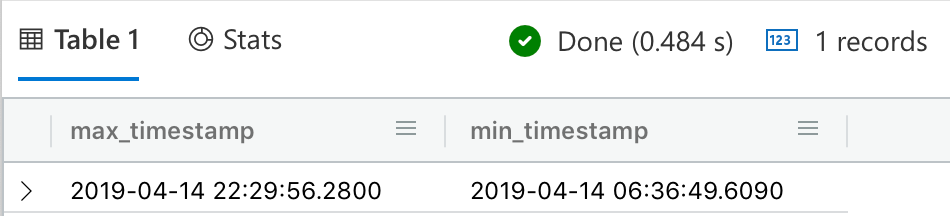 |
| Execution time: 93 ms |
Timescale
1
2
3
4
5
6
7
SELECT eventprocessedutctime FROM trucks
WHERE connectiondeviceid = 'd1626544-acfc-44fd-978a-6879f345a0da.truck-01.11578'
ORDER BY eventprocessedutctime DESC LIMIT 1;

SELECT eventprocessedutctime FROM trucks
WHERE connectiondeviceid = 'd1626544-acfc-44fd-978a-6879f345a0da.truck-01.11578'
ORDER BY eventprocessedutctime ASC LIMIT 1;
| Result |
|---|
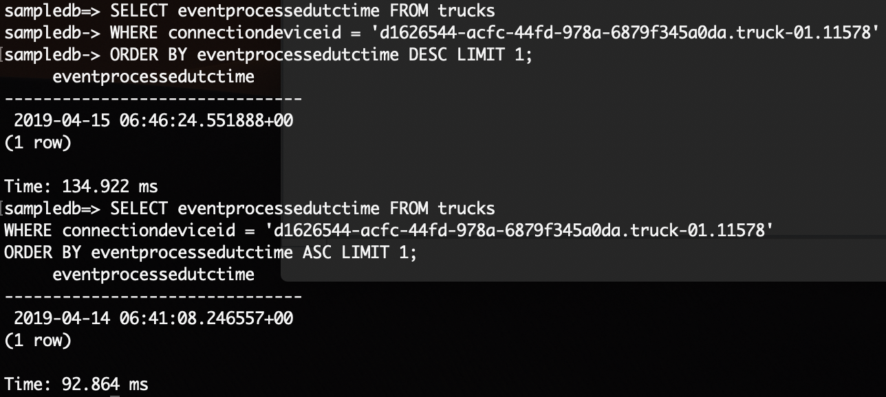 |
| 0.134secs and 0.092secs |
Both databases show a sub-500-millisecond performance. This shows that, when it comes to time-based queries, these databases are on fire and mean serious business.
Generic time series query, device-specific
The bread and butter of your database is going to be this query. It will return all messages sent by a specific device within a predetermined timeframe (in this case, a 4-hour time span).
columns cutout for brevity
ADX
1
2
3
4
5
let endtime = todatetime('2019-04-14T22:29:56.28Z');
let starttime = datetime_add('hour', -4, endtime);
Trucks
| where deviceId == 'd1626544-acfc-44fd-978a-6879f345a0da.truck-01.11578'
| where timestamp between (starttime .. endtime)
| Result |
|---|
 |
| Execution time: 778 ms |
Timescale
1
2
3
4
5
SELECT *
FROM trucks
WHERE connectiondeviceid = 'd1626544-acfc-44fd-978a-6879f345a0da.truck-01.11578'
AND eventprocessedutctime <= TIMESTAMPTZ '2019-04-15 06:46:24.551888+00'
AND eventprocessedutctime > TIMESTAMPTZ '2019-04-15 06:46:24.551888+00' - interval '4 hours';
| Result |
|---|
 |
| 0.692secs |
Binning
Binning is the most important feature you can get in your time series database. Your IoT application will be doing time bins everywhere. It is here where most databases fail to deliver. Binning is important for two reasons:
- Significantly reduces the load on your database and on your backend application
- Summarises loads of data in a way that is understandable to a human.
For those that did not read my first post in this series, binning intends to solve the following problem (if you already know what binning is, skip this paragraph). Suppose you have a device that sends a message every 5 seconds. Now, suppose the user consults the last 3 months of historical data. If you just query for all historical data for that device for the last 3 months, that query is going to return 1.5 million results. Your user won’t be able to interpret any of that data. Also, suppose you throw these 1.5 million results into a remote monitoring visualization dashboard. The graph is going to be cluttered and impossible to understand. Also, having a single query deliver 1.5 million results will put pressure on your database (in reality, you’ll have to page through results), your API, your client application and your network too. Binning allows you to do the following: “for all the data accumulated in the last 3 months, split the data into bins of 1 day. Calculate the average of the measurements on every bin, and return the result to the user”. Of course, you can define the length of the bins and the aggregation function you want to use.
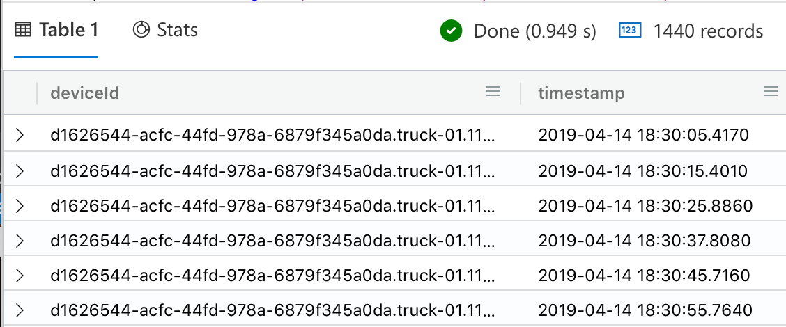
We are now going to run binning on both ADX and Timescale. We will do that for 1 deviceId, for a period of 4 hours, with bins of 30 minutes, and we’ll compute the average, min value and max value on every bin. We’ll be looking at the temperature value. But before we do that, we’ll simply count the number of messages for that period of time, just to get an idea about the size of the result set without binning.
ADX
1
2
3
4
5
6
7
let endtime = todatetime('2019-04-14T22:29:56.28Z');
let starttime = endtime - time(4h);
let interval = 30min;
Trucks
| where deviceId == 'd1626544-acfc-44fd-978a-6879f345a0da.truck-01.11578'
| where timestamp between (starttime .. endtime)
| summarize count()
| Result |
|---|
| 1,440 |
| Execution time: 0.132secs |
Timescale
1
2
3
4
5
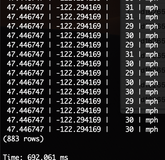
SELECT count(*)
FROM trucks
where connectiondeviceid = 'd1626544-acfc-44fd-978a-6879f345a0da.truck-01.11578'
and eventprocessedutctime <= TIMESTAMPTZ '2019-04-15 06:46:24.551888+00'
and eventprocessedutctime > TIMESTAMPTZ '2019-04-15 06:46:24.551888+00' - interval '4 hours'
| Result |
|---|
| 883 |
| 7.091secs |
We’ll later run binning across millions of rows, don’t worry. Let’s run the binning for this one device now:
ADX
1
2
3
4
5
6
7
let endtime = todatetime('2019-04-14T22:29:56.28Z');
let starttime = endtime - time(4h);
let interval = 30min;
Trucks
| where deviceId == 'd1626544-acfc-44fd-978a-6879f345a0da.truck-01.11578'
| where timestamp between ( starttime .. endtime )
| summarize avg(temperature), min(temperature), max(temperature) by bin(timestamp, interval)
Result

Execution time: 640 ms
Timescale
1
2
3
4
5
6
7
SELECT time_bucket('30 minutes', eventprocessedutctime) AS thirty_min, avg(temperature), min(temperature), max(temperature)
FROM trucks
where connectiondeviceid = 'd1626544-acfc-44fd-978a-6879f345a0da.truck-01.11578'
    and eventprocessedutctime <= TIMESTAMPTZ '2019-04-15 06:46:24.551888+00'
    and eventprocessedutctime > TIMESTAMPTZ '2019-04-15 06:46:24.551888+00' - interval '4 hours'
GROUP BY thirty_min
ORDER BY thirty_min DESC
Result
1
2
3
4
5
6
7
8
9
10
11
       thirty_min | avg | min | max
------------------------+---------------------+--------+--------
 2019-04-15 06:30:00+00 | 31.2952622950819672 | 29.969 | 32.406
 2019-04-15 06:00:00+00 | 34.4474181818181818 | 31.084 | 37.441
 2019-04-15 05:30:00+00 | 35.4402181818181818 | 33.909 | 37.544
 2019-04-15 05:00:00+00 | 36.2109636363636364 | 34.097 | 37.976
 2019-04-15 04:30:00+00 | 35.0598288288288288 | 33.891 | 37.511
 2019-04-15 04:00:00+00 | 34.0196576576576577 | 33.018 | 35.255
 2019-04-15 03:30:00+00 | 35.0200181818181818 | 33.726 | 36.065
 2019-04-15 03:00:00+00 | 35.9602252252252252 | 34.325 | 37.834
 2019-04-15 02:30:00+00 | 35.3813061224489796 | 34.445 | 36.455
Execution time: 221 ms
Now let’s remove the filter on deviceId and see how binning behaves across millions of rows of data:
ADX
1
2
3
4
5
6
7
let endtime = todatetime('2019-04-14T22:29:56.28Z');
let starttime = endtime - time(4h);
let interval = 30min;
Trucks
//| where deviceId == 'd1626544-acfc-44fd-978a-6879f345a0da.truck-01.11578'
| where timestamp between ( starttime .. endtime )
| summarize avg(temperature), min(temperature), max(temperature) by bin(timestamp, interval)
Execution time: 635 ms
Timescale
1
SELECT time_bucket('30 minutes', eventprocessedutctime) AS thirty_min, avg(temperature), min(temperature), max(temperature) FROM trucks where eventprocessedutctime <= TIMESTAMPTZ '2019-04-15 06:46:24.551888+00' and eventprocessedutctime > TIMESTAMPTZ '2019-04-15 06:46:24.551888+00' - interval '4 hours' GROUP BY thirty_min ORDER BY thirty_min DESC;
Execution time: 5.508 secs
If your database does not offer binning support, you’ll have to retrieve the entire result set from your database, and do the bins in your own application code. You’ll never achieve the performance seen above. Plus, we are lazy developers, we don’t want to write code unless we absolutely have to, right?

One drawback of binning is that it will smooth out the data and it will be hard to spot anomalies. That’s why I typically provide binning with more than 1 dimension. In the case above, I am computing the average, the min and the max values. The average value will allow you to understand the trend of your devices. Whereas the min and max values will help you spot anomalies. You can use other aggregation functions (such as standard deviation) to dig into the data. In any case, if you spot a specific bin which looks funny, you can always query the entire dataset for that specific bin only (remove the aggregations).
For your benefit, this is how the query above would look like to a user with binning:

And without binning:
 Even the database itself tells you that this query is a BAD idea…
Conclusion
I hope to have demonstrated some of the most common IoT data access patterns we find in our projects, as well as how to implement them using Azure Data Explorer and Timescale.
Trying to implement these queries on large datasets on databases which are not optimized for time series is costly, suffers from slow performance, and takes more development effort. Therefore, you should invest time in selecting the right database for your IoT use case.
I want to finish with a note about ADX and Timescale. The purpose of these blog posts is not to compare ADX vs Timescale and decide which one is faster/better/etc. So don’t take these posts as a showdown between the two. However, people have asked what are the advantages of one over the other, or what the selection criteria are to choose between them.
Timescale
In essence, Timescale is still an RDBMS. It builds on top of PostgreSQL, which is a relational database. Wait a minute… didn’t I say in my first post to avoid RDBMS for IoT scenarios? In fact I did, but Timescale is an optimization for time series on top of PostgreSQL. However, by looking at the performance of some of the queries above, you can see that sometimes the limitations of the relational architecture show up. The performance for counting is terrible. Typically, aggregations will perform lower compared to a database like ADX. Timescale users will usually create aggregation views on top of the telemetry tables they use to accelerate performance. When it comes to time series data, PostgreSQL is a huge improvement compared to the incumbents, such as MS SQL, Oracle or the likes. But it won’t match the performance and capabilities of a hyperscale architecture like ADX. Postgres will run on-prem, for example, if you need to keep a database at the edge for a historian or another purpose where cloud connectivity is a problem or an overkill. You can also benefit from the fact that it’s a relational database, meaning you can have other tables in the database and join them with telemetry data.
ADX
ADX uses a completely different architecture from relational databases, and you can see what that means in performance. Simply put, the performance of ADX is criminal. Specially when it comes to aggregations across billions of rows, I’ve seen ADX perform in datasets much much larger than the 113 million rows I used for these blog posts, and its performance never ceases to amaze me. It’s a product built for hyperscale and hyperperformance. It’s a product built for a scale your own organisation will probably never see (as a matter of fact, the product’s origins inside Microsoft date back to the need of handling all the telemetry and diagnostics data Azure services were generating. A problem of apocalyptic scale, considering the scale of Azure). ADX is not for everybody though. First, ADX is propietary IP from Microsoft, which means it runs in the Azure cloud only. If your organization already has an investment and commitment to Azure, then that’s alright. But if you’re invested in another cloud, or still want to run on-prem, ADX is not the right database for you. ADX also requires your team to learn another query language (KQL - Kusto Query Language). The language is super intuitive and delightful to use, yet most people are already used to SQL and adopting ADX means your team will have to go through a slight learning curve.
Acknowledgements
Again, many thanks to the wonderful people at the Microsoft ADX team for their comments, feedback, and suggestions.
Also, many thanks to the people in the community of Timescale. In particular, they have a quite active Slack group, which is public and open to anybody, where people contribute content, ideas and help each other solve problems.